Tech Stuff - Digital Sound Primer

This primer describes the process of digitizing analog sound for use in processing systems (that's a PC for most of us, but could be a specialized workstation or a DSP). It is a companion piece to an overview of notes, harmonics, overtones and all that stuff that you need to be comfortable with before you even start thinking about digital sound. There are multiple digital sound documents all over the web. Some are very good. But most stop when it starts to get really interesting.

Contents

1. Analog Sound Stuff (mercifully short)
2. 'Ish Recording History (rough dates for various events in the recording world)
3. Digitizing Sound (bits and bytes)
4. Time Domain and Frequency Domain (inside the digital samples)
5. ADSR and Harmonics (real life examples)

Analog Sound: A Lot of Pushing and Shoving

Sound travels in pressure waves. The sound source, say, a loudspeaker vibrates which starts to push the air molecules at its surface and these air molecule guys push the next air molecule guys and so on for as long as they have enough energy left - pushing air molecules around is hard work and they don't get paid much. Sound pressure waves travel at a speed of somewhere around 1,236 Km/hour (768 mph). It varies slightly depending on altitude - there are less of these air molecule guys to push around at higher altitude so sound travels slightly slower. So if you get to the top of Everest and have any breath left it will take your friends back home a bit longer to hear your victory shout than it would if you had only climbed a modest ladder - which is another good reason not to climb Everest if you were looking for one.

The speed of sound is the same whether you whisper or yell at the top of your lungs. When you whisper you are not providing much energy and all that pushing and shoving of air molecules will soon stop, whereas, if you shout then you provide a lot of energy and these happy little air molecule will have a rare old time pushing and shoving their neighbours for quite some time - and hence the sound will cover a lot more distance.

Most systems that generate sound, for example, a loudspeaker, your mouth, or a trumpet, are directional and the sound waves start by scampering off in the direction in which they are pointed. Then, poor devils, they tend to bump into things - like walls and people and blades of grass. When they do this they bounce off in fairly random directions and may then bump into something else until they are finally overcome with exhaustion or arrive at a sound receiver such as an ear or a microphone. So the ordered picture of well behaved sound waves marching off into the distance like little toy soldiers is pretty misleading. Instead these sound waves are more like drunken louts staggering around and bumping into things until they finally collapse. Quite sad really. But occasionally useful, since all this bumping around is the reason that someone standing behind you can occasionally hear what you say - which might not always be a good thing.

All this bumping and bouncing around also explains the difference between listening to music on your down-and-dirty stereo system at home and listening to the exact same performance in a major concert hall. The sound waves are bouncing off things (highly technical term) in different ways and thus get to your ears (or some transducer - such as a microphone) at different times. However, it also suggests that we could, perhaps, process the recorded sound - using a process generically called signal processing - to modify the time at which the recorded signals are sent from your loudspeaker in such a way that they sound as if they were happening in a major concert hall. So we could delay the violins a bit, bring the cellos forward in time, bump up the timpani etc. And if we were sufficiently smart perhaps we could even match the sound profile of a specific concert hall, for example La Scala, Milan, assuming you were sitting in row H seat 12. This is the basic idea behind what is sometimes called surround sound.

Recording History: Sing Louder...

Recordings of sound were made as early as 1857 but the first viable reproduction systems date from around 1870. The following is a rough guide to what happened, and when, on the road to digital sound. It is not meant to be accurate to the week - there are plenty of excellent resources on the web that will give you precise histories of most of the individual items - but rather to give a overview of when'ish certain things happened on the way to digital audio.

The 'ish History of Sound Recording

Cylinders	1880s'ish	Wax coated cylinders individually copied from a master. Continued in production until the late 1920s.
Flat Discs	1895'ish	Originally hard rubber flat discs stamped from a master. By early 1900's flat discs were the dominant technology and Shellac had replaced hard rubber. Various incompatible playback speeds were used. 7 to 12 inch record sizes.
Acoustical Recording	1880s'ish	Recordings (on either cylinders or discs) were pure mechanical-acoustical using a horn to focus the sound which mechanically operated a cutting stylus. Acoustic recording made it almost impossible to record drums since the vibrations could cause the cutting stylus to jump. Violins required special amplifying horns and cellos and double bases where generally too quiet to record well. Singers had to stand close to the horn and were frequently told to sing louder. All playback systems until the late 40's and well into the 50's were purely mechanical - clockwork driven systems that had to be hand-cranked between records.
Electrical Recording	1924'ish	Electrical recording , developed originally by Western Electric, was made possible through amplified microphones which drove the mechanical recording stylus in their first incarnations. Within a year or so of its introduction it had largely replaced acoustical recording. Electric playback systems (record players) originally appeared around 1933 but did not achieve any consumer market penetration until the late 40's and well into the 50's. Prior to that they were limited to juke-boxes and similar devices.
78 RPM Discs	1925'ish	78 RPM, 10 or 12 inch, Shellac discs became the industry norm from around 1925 with 12 inch eventually becoming dominant. 78's continued in production until 1959 - 1961.
Vinyl Discs	1933'ish	While experimental vinyl records were made in the 1930's it was not until the advent of the LP (1948'ish) that they became the industry norm.
Digital Sound	1943'ish	The earliest operational systems using digital sound date from this period and used what became known as Pulse Coded Modulation (PCM) which is still the basis of digital sound. The original work was carried out for the telephone system and exploited for use in war-time communications. It would be the 1980's before digital playback systems became consumer items.
LP (33 RPM)	1948'ish	Originally produced in 1948, by 1952 12 inch vinyl LPs became the norm (though some 10 inch versions were also produced). 20 - 30 minutes playing time on each side.
Single (45 RPM)	1949'ish	Originally produced in 1949, by 1954 7 inch vinyl singles had sold over 200 million copies. Singles had two 4 minute sides. Extended Play (EP) records, with a total of 5 - 8 minutes playing time per side (total of 4 songs), were also issued as 45's.
Stereo Records	1958'ish	Originally invented and prototyped in 1931 the 45 degree stereo record was not commercially produced until the late 50's using the Westrex system developed by Western Electric. Prior to their use in records, stereo techniques were confined mostly to use in the film world.
Digital Recording	1976'ish	Initially used to simply store sound data in digital format which was then used to create masters for LP's or Singles. Mixing and filtering of digital audio did not occur until well into the 80's.
CD	1982'ish	First commercial digital playback system. Optical media. Standard Red Book CD is 80 minutes playing time (700 MB data). Standardized as 44.1 KHz sample rate (giving a maximum frequency range of 22.05 KHz) all CDs contain a filter which eliminates everything above 20 KHz on recording and playback. The sample-size (a.k.a bit-depth) is 16 bits. Dynamic range is 96dB. Encoding uses LPCM (Linear pulse Coded Modulation).
DVD	1995'ish	Optical media. Multiple variations within the standard. Allows for 16-bit and 24-bit sample-size and sample-rates up to 192 KHz. Not common for digital audio. Whereas the Video DVD is near ubiquitous.
SACD	1999'ish	Super Audio CD. Optical media. Uses a 1-bit DSD (Direct Stream Digital) sample-size (vs 16-bit for CD) and a sample-rate of 2822.4 KHz (vs 44.1 KHz for CD). No we did not make this up. Most SACDs are hybrids which have both a classic CD and SACD recordings on the same media. Conventional CD players pickup only the CD. The enhanced SACD capabilities require an (expensive) SACD player. Not yet widely adopted.

Digitization: What a lot of Samples

Sound is digitized by sampling the amplitude (strength, measured in Volts) of a waveform from a capturing device (a.k.a a transducer - typically a microphone) using an ADC (Analog to Digital Converter). In tech speak the process of creating the sample using an ADC is called quantization. The sampling is performed at a particular rate (the sampling rate) expressed in samples per second. Sampling (Nyquist) theory says that to digitize a signal effectively it must be sampled at twice its maximum frequency, that is, twice the frequency of the highest frequency (Notes, harmonics, overtones etc.) that can appear in the sound source. If a lower sampling frequency is used the peaks or troughs can occur between sample times. At twice the maximum frequency peaks and troughs cannot be missed between samples simply because they cannot occur. The resulting digital samples from this quantization process are said to be in the Time Domain. The samples will produce a Time Domain waveform which is a plot of amplitude (vertical or Y axis, captured in Volts) versus time (horizontal or X axis) as shown in the Figure 1. (Figure 1 was created using the excellent Open Source Audacity audio editor using an MP3 audio file - which was, in this case, ripped from a CD.)

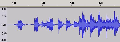
Figure 1 - Time Domain Waveform

Figure 1 shows the Time Domain waveform when an audio file is loaded into Audacity - any file format (WAV, AAC etc) will look like this we just happen to have used an MP3. It is not a sound wave but a digital representation of a waveform that will produce sound (sound waves) when it is played through loudspeakers via, say, a PC card (which is not much more than a Digital to Analog Converter or DAC). It is called a Time Domain waveform simply because it graphs time on the horizontal (or X) axis - in Figure 1 the time values from 1.0 to 4.0 seconds are visible - against amplitude on the vertical (or Y) axis - in Figure 1 amplitude ranges from 1.0 at the top to -1.0 at the bottom.

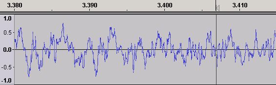
Figure 2 - Time Domain Waveform - Expanded

Using Audacity's zoom feature Figure 2 shows an expanded view of the Time Domain waveform centered at around 3.4 seconds (the black vertical line is Audacity's audio cursor). How all this magical stuff happens can be seen by zooming in further (using the same center line) as shown in Figure 3.

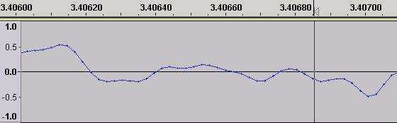
Figure 3 - Time Domain Waveform - Sampling Points

We have zoomed in so that we can now see the individual samples in the Time Domain wave form (the little dots on the wave each represent an individual sound sample - the lines joining the dots are added by the software - Audacity in this case - simply to allow we simple humans to 'see' or visualise an approximation of the waveform).

So what are these samples and where do they come from? A digital sound sample is a numeric value representing the amplitude of the electrical waveform originating from the sound capture device (typically a microphone) and taken at particular points in time (the sample-rate). The normal range of human hearing is from a frequency of around 20 Hz to around 20 KHz. To capture all the sound we can hear, sampling theory says we must sample at twice the maximum frequency we want to capture. This would mean sampling at a minimum of 40 kHz (2 x 20 kHz) or 40,000 times per second. In practise the waveform (shown in Figures 1 - 3) is from a CD which, when encoded, is sampled at the slightly higher rate of 44.1 kHz or 44,100 samples per second for purely historic reasons. Each of the sound samples (the dots) shown in Figure 3 thus represents 1/44,100 of a second. Note: A 44.1 kHz sampling frequency means that we can theoretically capture frequencies up to 22.05 kHz (sampling frequency/2). However, the CD specification defines a cut-off filter which kills all sound above 20 kHz meaning there is no useful sound material above 20 kHz in digital sound.

So what have we sampled?

Each sound sample was captured by an Analog to Digital Converter or ADC in a process called quantization and represents the amplitude (strength) of the electrical signal (in volts) coming from a transducer (typically a microphone) used to capture the sound. The accuracy of the sample (and thus its quantization error) is determined by the sample size (a.k.a. bit depth). The larger the sample size the greater the accuracy of the sample, or if you prefer it in negative terms, the larger the sample size the lower the quantization error. In the case of a CD the sample size is always 16 bits, for a DVD it may be 16, 20 or 24 bits. When using 16 bits, as in the CD case, each sound sample may take one of 65,536 (0 to 65535) possible values to represent the amplitude value in volts (65536 is the maximum decimal number that can be contained in 16 bits). This range of amplitude values gives a very good approximation of the real sound when it is played back and indeed there are those who assert that for playback purposes 16 bits is more than adequate to cover the full audible range at high quality levels. If, however, the sample size was only 8 bits this would give only 256 (0 to 255) possible values and give a poor approximation of the original signal (entirely due to large quantization errors) and hence a pretty lousy playback quality. If, on the other hand, a 20 bit sample-size was used this would yield 1,048,576 (0 to 1048575) possible values giving a more accurate approximation of the original analog waveform - simply by reducing the size of the quantization errors. In general, higher sample rates (> 16 bits) make sense during recording or capturing sound material to create 'masters' whereas 16 bits gives more than acceptable playback quality.

This long article makes an agressive case against the need for higher sample-sizes as well as providing a good overview of how the human ear works.

To summarize: the sample-rate controls the frequency range that we can capture and the sample-size controls the accuracy of each sample.

When sound is captured in this manner it is called Pulse Coded Modulation or PCM (more properly LPCM) and originates from early work on digitization of the phone network. The sample numbers coming from the ADC are always positive and the zero level (see Figure 3) is assumed to be sample size divided by two. Thus a 16 bit sample has a maximum range of 65,536 (32767 to -32768) and numbers above 0 are plotted on the positive (upper) side of the Y axis and below 0 are plotted on the negative side. The sample values obtained are relative (or dimensionless) to the capture and playback systems - they are shown on a 1.0 to -1.0 scale in Audacity and most other audio editors simply to make them comprehensible. This dimensionless scale makes sense when you consider that transducers (capture devices, for example, a microphone) vary widely in their sensitivity, normally measured in mV/Pa (milli volts per Pascal), and may have a range as high as +-10V (in professional configurations) whereas when played back through a conventional PC sound card, which converts from the sound sample to a voltage using a Digital to Analog Convertor (DAC), the maximum output voltage is typically 2V. In one case the value +1.0 (on Audacity's scale) may have a real world value of +10V (professional microphone input) and in the other case +2V (PC loudspeaker output). It is the ADC or DAC that does the real world to digital world conversion.

Frequency Domain: Where's my Notes

The waveform that is digitized and shown in Figure 4 represents the Time Domain. The amplitude of the signal originating from a transducer (usually a microphone) at particular points in time - defined by the sample rate which, in the case of Figure 4, is 44.1 KHz because it originates from a CD.

This Time Domain waveform in Figure 4 is a piece of music. And we all know that musicians play notes like C4 or A3# etc. when they hit things, blow into things or saw things. And notes are sound frequencies and have harmonics and overtones and all that good stuff. So where did all the frequencies go?

Figure 4 - Time Domain Waveform

The Time domain waveform in figure 4 is the sum of all the sound frequencies present in the signal. If we want to see the individual frequencies then we need to convert the waveform from the Time Domain to the Frequency Domain. To do this we need a little help from a French mathematician called Joseph Fourier and his theories that, very simply stated, say you can decompose a time domain into a frequency domain (and vice versa) by using a transform (specifically the Discrete Fourier Transform - DFT - a gruesomely complex mathematical alogorithm). Because we can also take certain shortcuts in performing this transform we typically use what is called a Fast Fourier Transform (FFT) algorithm. In essence, the FFT can be used to decompose a time domain set of digital samples into the consituent frequencies present (and their amplitude). Now if your brain is hurting - as indeed is ours - you can simply look at the results of this FFT process for the complete waveform shown in Figure 4 using another of Audacity's seemingly endless miracles.

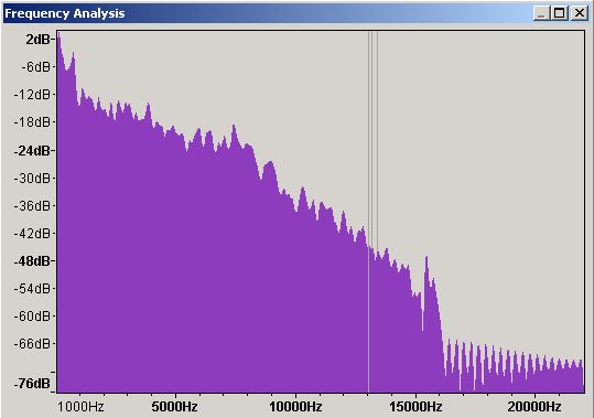
Figure 5 - Frequency Domain Spectrum Analysis - Linear Scale

Figure 5 is a spectrum analysis (a.k.a. a frequency analysis) of the whole waveform shown in Figure 4. This particular format is called a linear display simply because it uses equally spaced frequency graduations on the X axis - from 1,000 Hz (1 KHz) to 20,000 Hz (20 KHz) - in Figure 5. The vertical (Y) axis shows the sound level of the various frequencies measured in decibels (dB) which is kinda related to their loudness when played back. This particular plot shows a maximum output value of 2 dB (which we will see later may cause output sound distortion) somewhere below 1000 Hz (or 1 KHz).

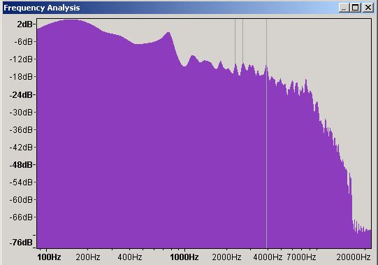
Figure 6 - Frequency Domain Spectrum Analysis - Logarithmic Scale

Figure 6 shows the same frequency domain plot but displayed on a logarithmic scale - simply a way of handling large number ranges with lots of detail at the low end and progressively less at the higher end so the scale in this case goes from 100 Hz to 20,000 Hz (20 KHz) with the numbers at the top much closer together. In this plot it is now clear that the peak of 2dB is around 150 Hz and will probably create a big bass thump on the speaker - if it's a badly designed speaker it may even fall over. Which type of plot you use, linear or logarithmic, is largely a matter of taste but recall that humans are more sensitive to sounds in particular frequencies (roughly 400 Hz to 3 KHz) than in others. The log plot covers the whole of this range the linear plot does not.

Finally, all of these plots are averages of the amplitude (dB) over the selected time period of the plot. That is to say the average value of the frequency peak at around 150 Hz is 2dB - if there are multiple occurrences of 150 Hz frequencies - if - then some may be higher and some lower or they could all be 2dB. There is not enough data in the plot to say which of these scenarios is true.

Don't really believe all this hidden stuff? If you want to see time domain to frequency domain stuff in action this great java applet animates the process.

It's All Just Noise (Distortion)

There are a couple of points we need to get out of the way at this stage. Sounds can be distorted in a variety of ways. The term clipping is an analog audio term that refers to sounds out of the range that the equipment can handle. It is applied to both input and output signals. In the digital world lets take them one at a time.

When recording through a digital interface the microphone (say) will generate an electrical signal (a continuously varying Time Domain waveform) which is the sum of all the sound frequencies it is receiving. The ADC (a PC soundcard or other digitization system) will sample this waveform. If the sound card expects a maximum to minimum range of +2V to -2V and the microphone is generating +10V to -10V we are going to miss all the data above +2V and below -2V. If the microphone voltage range is lower than that of the digitization system, say +1V to -1V, then we are going to get very quiet input. The microphone and digitization system outputs/inputs ideally should be perfectly matched. The world ideally is important here. In our 10V microphone case if the sound that we actually want to capture always occurs within the range +2V to -2V we are OK. Similarly in our 1V case we could always digitally amplify the input signal (but thereby also introduce a possible distortion).

Time Domain output. The sound samples of the Time Domain waveform are, as we have seen, simply numbers. They can be manipulated like all numbers. Amplification (volume control) is nominally a process of multiplying the sound sample by some desired value. If, however, in a 16-bit system we multiply a sound sample with a value of 40227 (valid) by 2 we get 80454 which is in excess of the maximum value of 65536 for a 16 bit system. The sound sample in this case is clipped and when actually output could either be set to the maximum value (65535) or wrapped (80454-65536 = 14918). Most digital sound editing software will prevent this condition or at least indicate that it has happened.

Distortion of sound output can also occur when a frequency (in the Frequency Domain obviously) is output with a greater sound power (in dB on our Frequency Domain plots) than the sound system (loudspeaker) is capable of handling, or, in the jargon, for which the speaker does not have a good frequency response - meaning the speaker rattles or exhibits some other unpleasant behavior. The maximum figure for any frequency in the digital domain is 0dB (or for safety many system limit this to -5dB) - in the case of certain speakers (cheap ones especially) it may be much lower at certain, or even all, frequency ranges.

The relationship between Time Domain waveform amplitude and Frequency Domain amplitude is - essentially - non-existent. The following is an Audacity waveform of a 200 millisecond section of music.

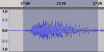
Figure 7 - Time Domain waveform

Nothing too exciting about the waveform and well within the clipping limit. However...

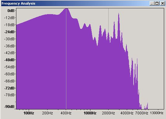
Figure 8 - Frequency Domain waveform

This is the frequency domain plot of the same 200 millisecond period and shows that the frequency around 400 Hz is showing 0 dB which can lead to loudspeaker distortion. All is not as it seems. Both time and frequency domains are important. Now to illustrate the relationships we are going to try some experiments.

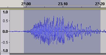
Figure 9 - Time Domain waveform - EQ Boosted

Using the equalization feature of Audacity (yet more magic) we boost the value of the 400 Hz frequency range. Figure 9 is the resulting waveform which has increased in amplitude but is still well below the clipping limit of 1.0.

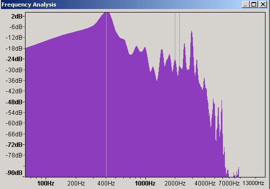
Figure 10 - Frequency Domain waveform - EQ Boosted

Figure 10 is the frequency plot (of the time domain sample in Figure 9) showing that we now have a peak of 2 dB (up from 0 dB) and which will now most likely cause some distortion. We undo the change (yet another audacity feature) and amplify the selected section (you guessed using another Audacity feature) by 5 in this case (Audacity allowed us to amplify to 5.7 only in this case to prevent clipping).

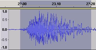
Figure 11 - Time Domain waveform - Amplified

The time domain plot (Figure 11) is now much bigger (because amplify works on all frequencies - whereas our equalization change was applied only to a very narrow band of frequencies around 400 Hz) and is approaching the clipping limit.

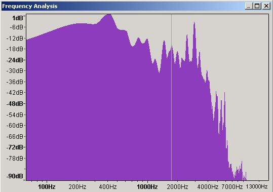
Figure 12 - Frequency Domain waveform - Amplified

When we plot the frequency domain (Figure 12) we now have a 400 Hz frequency with a peak of 1 dB which will probably cause modest distortion on all but the very best speakers. The law of unintended consequences is alive and well.

It's All a Question of Scale

If you can handle a little more pain it is worth looking at frequency plots in a little more detail to understand their limits. We wrote earlier that the frequency plots use a Fast Fourier Transform (FFT) algorithm and that the plots were an average of the frequency over the plot time selection period. The FFT algorithm can be used with varying degrees of accuracy - Audacity's default is 512 which is the value used on all the plots above. The following plots show the same selection period at 512, 1024, 4096 and 16,384 accuracies.

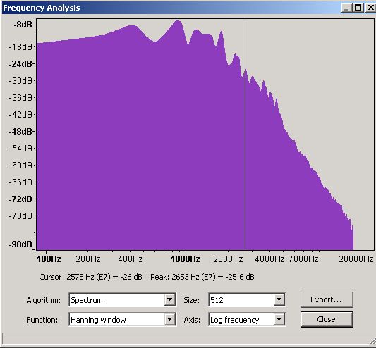
Figure 13 - Frequency Domain - 512 slots

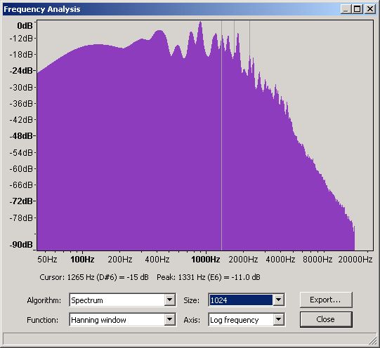
Figure 14 - Frequency Domain - 1,024 slots

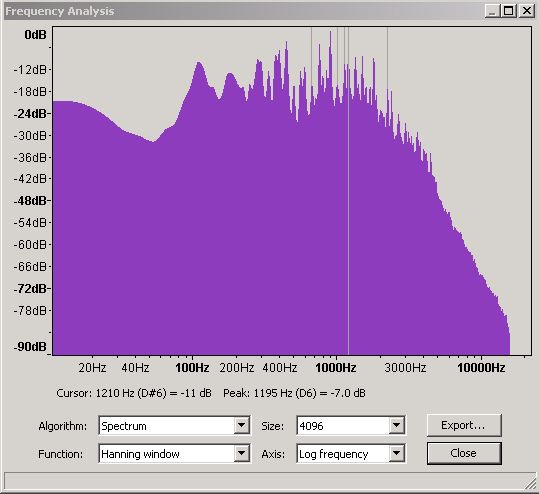
Figure 15 - Frequency Domain - 4,096 slots

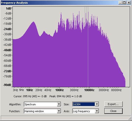
Figure 16 - Frequency Domain - 16,384 slots

ADSR: Who Hit What

Each musical note has a defined frequency. However, if we play the same note, say C4 (middle c) on a piano and a saxophone even to our untrained ears it sounds different. An instrument's characteristic sound (or timbre) is determined by its ADSR or Amplitude Envelope. The ADSR exists in the Time Domain. Figure 17 shows the Time Domain ADSR for a piano playing C4 (middle C) which has a frequency of 262 Hz.

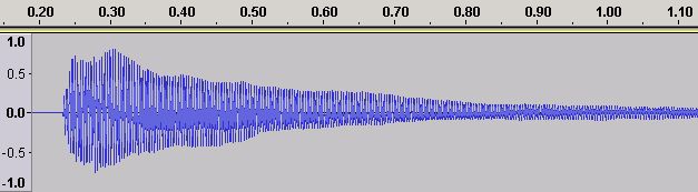
Figure 17 - Time Domain ADSR for a Piano Middle C (C4)

The note sample in figure 17 is from the astounding collection made freely available by the University of Iowa (unfortunately the site was not available the last time we checked) and was played on a Steinway Piano and recorded in Stereo (a mono and slighly amplified version is shown for visibility reasons). Different brands and even models of piano will have (minor) variations on this ADSR.

Figure 18 shows the Frequency Domain at 4096 slots for this ADSR and allows us to see the harmonic characteristics of this particular piano. Again, different models and makes of piano will exhibit varying degrees of difference.

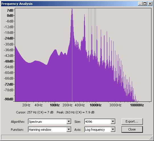
Figure 18 - Frequency Domain for a Piano Middle C (C4)

From this graph and using Audacity's measuring tool gives readings of:

Harmonic	Frequency	dB	db (%)
1st (Fundamental)	262	1.2	100%
2nd	525	-4	96%
3rd	788	-16	84%
4th	1051	-16	84%
5th	1317	-19	81%
6th	1583	-17	83%
7th	1849	-14	86%

Figures 19 and 20 show the Time Domain and Frequency Domains for the note B3 (the note below middle C) on the same piano.

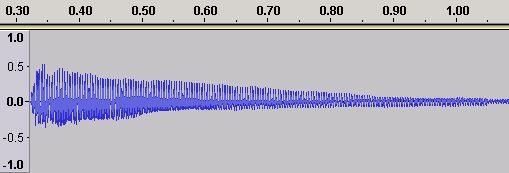
Figure 19 - Time Domain ADSR for a Piano B3

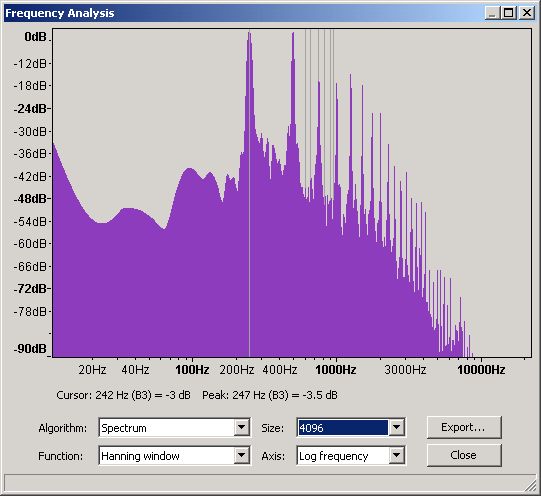
Figure 20 - Frequency Domain for a Piano B3

From this graph and using Audacity's measuring tool gives readings of:

Harmonic	Frequency	dB	db (%)
1st (Fundamental)	247	1.3	100%
2nd	496	1.1	100%
3rd	743	-19	81%
4th	992	-10	90%
5th	1243	-4	96%
6th	1492	-8	92%
7th	1746	-10	90%

The following 4 Figures show the equivalent Time and Frequency Domains for a violin and are taken from the same University of Iowa collection. The samples have been amplified from the originals purely for the sake of presentation.

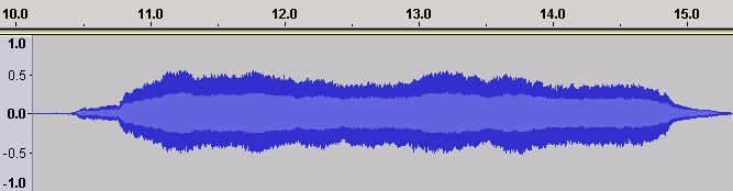
Figure 21 - Time Domain ADSR for a Violin Middle C (C4)

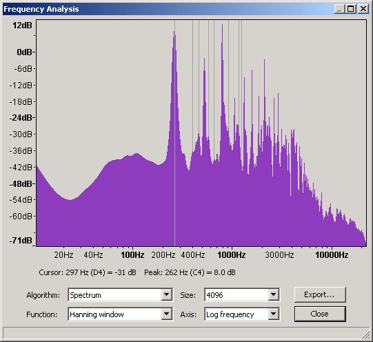
Figure 22 - Frequency Domain for a Violin Middle C (C4)

From this graph and using Audacity's measuring tool gives readings of:

Harmonic	Frequency	dB	db (%)
1st (Fundamental)	262	8	100%
2nd	523	-2	94%
3rd	786	11	103%
4th	1047	-14	78%
5th	1308	-4	92%
6th	1571	-4	92%
7th	1833	-10	82%

Figures 19 and 20 show the Time Domain and Frequency Domains for the note B3 (the note below middle C) on the same piano.

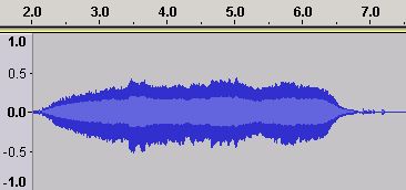
Figure 23 - Time Domain ADSR for a Violin B3

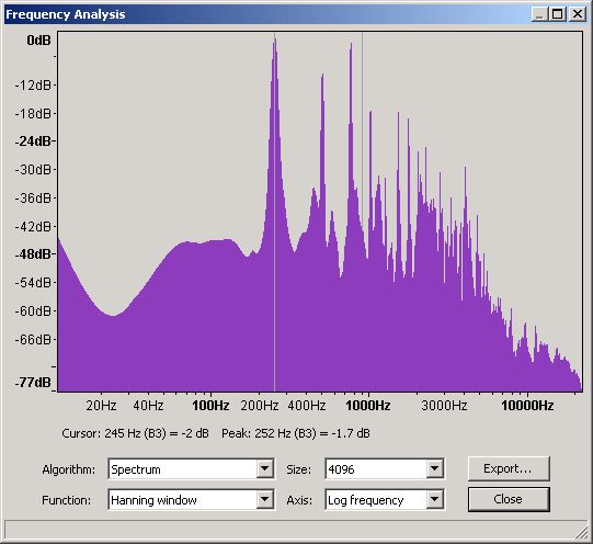
Figure 24 - Frequency Domain for a Violin B3

From this graph and using Audacity's measuring tool gives readings of:

Harmonic	Frequency	dB	db (%)
1st (Fundamental)	252	7	100%
2nd	505	0	93%
3rd	757	-8	102%
4th	1008	-2	91%
5th	1260	-20	73%
6th	1513	-4	89%
7th	1766	-0	93%

Notes about ADSR Values:

1. Only a single sample of each note is provided by the University of Iowa library of sound samples. The obtained figures may therefore be regarded as 'order of magnitude' correct rather than precisely measured.

2. The piano sample frequency values are closer to those provided in notes by frequency table than those of the violin. This may be explained by the more precise mechanism of a piano whereas a violin requires human judgment in selecting where on the string to place the bow. Additionally the Iowa samples do not indicate the tuning (though all the shown samples were played on the G string).

3. There are apparent discrepancies between the visible graph and the measurements taken using the Audcity tools. In all cases the measurements in the above tables were obtained by moving Audacity's audio cursor and noting the displayed values. However, it is also assumed, as a current hypothesis, that the dB values shown are less important than the relationship between them (shown in the % column).

To be continued - One Day Real Soon Now ™

---

Problems, comments, suggestions, corrections (including broken links) or something to add? Please take the time from a busy life to 'mail us' (at top of screen), the webmaster (below) or info-support at zytrax. You will have a warm inner glow for the rest of the day.